Visualizing differential equations or ODEs helps to better understand the behaviour of models. Especially in the special cases where limits are examined this visualisation makes things a lot easier.
With the following code you can easily plot them in Matlab. The important step is that have to norm the gradient in each point of the vector field. This can be achieved by using the command ones.
clear;
clf;
% creates grid points in the tp-plane
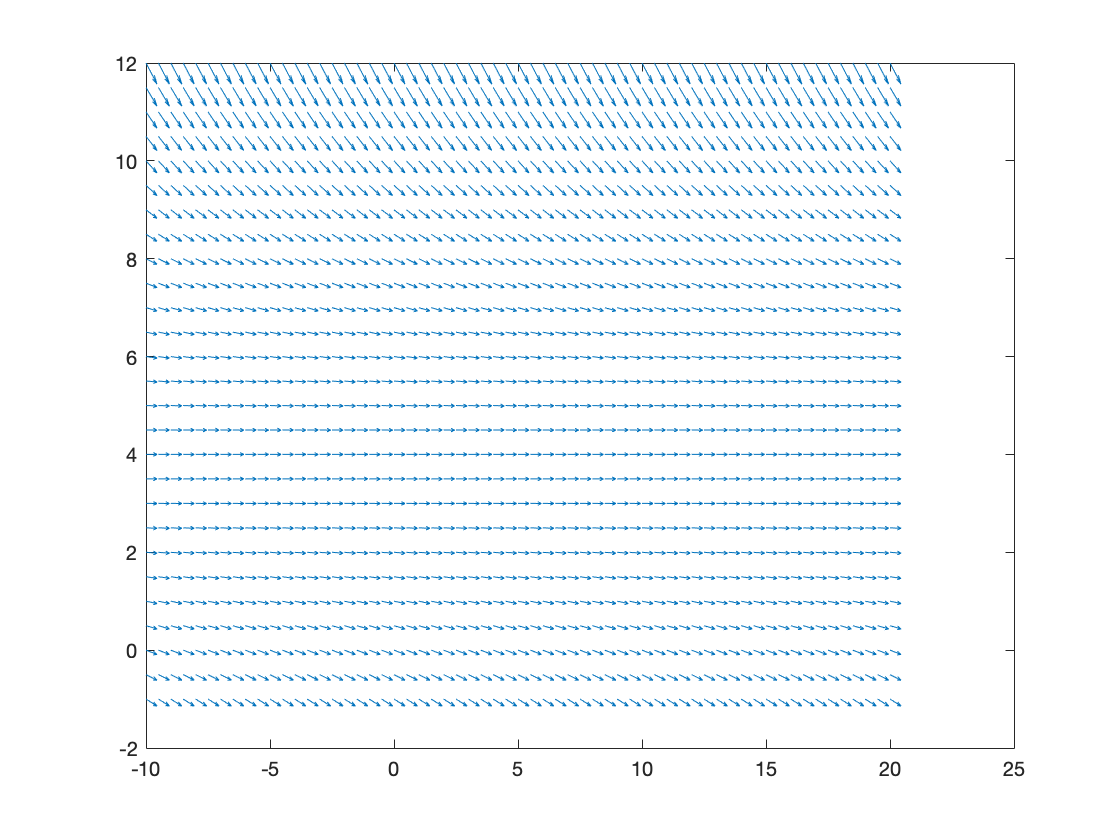
[t, p]= meshgrid(-10:0.5:20,-1:.5:12);
r = 0.2;
k = 7;
l = 2;
slope = -r.*(1-(2*p)/k).*(1-p/(2*l));
% plots direction vectors at all grid
quiver(t,p,ones(size(t)),slope)
Our function in this case: $$\dot{p} = -r (1 - \frac{2p}{k})( 1 - \frac{p}{2l})$$
You will get the following visualisation: